Statistic Methods Example

Functions and packages

library(knitr)

## Warning: package 'knitr' was built under R version 3.6.1

library(ggplot2)

## Warning: package 'ggplot2' was built under R version 3.6.3

library(RColorBrewer)
library(reshape2)

## Warning: package 'reshape2' was built under R version 3.6.1

library(formattable)

## Warning: package 'formattable' was built under R version 3.6.1

library(rms)

## Loading required package: Hmisc

## Warning: package 'Hmisc' was built under R version 3.6.3

## Loading required package: lattice

## Loading required package: survival

## Warning: package 'survival' was built under R version 3.6.3

## Loading required package: Formula

## 
## Attaching package: 'Hmisc'

## The following objects are masked from 'package:base':
## 
##     format.pval, units

## Loading required package: SparseM

## 
## Attaching package: 'SparseM'

## The following object is masked from 'package:base':
## 
##     backsolve

library(htmlTable)

## Warning: package 'htmlTable' was built under R version 3.6.1

library(cqsR)

## Loading required package: data.table

## Warning: package 'data.table' was built under R version 3.6.1

## 
## Attaching package: 'data.table'

## The following objects are masked from 'package:reshape2':
## 
##     dcast, melt

## Loading required package: VariantAnnotation

## Loading required package: BiocGenerics

## Loading required package: parallel

## 
## Attaching package: 'BiocGenerics'

## The following objects are masked from 'package:parallel':
## 
##     clusterApply, clusterApplyLB, clusterCall, clusterEvalQ, clusterExport, clusterMap, parApply, parCapply, parLapply, parLapplyLB, parRapply, parSapply, parSapplyLB

## The following object is masked from 'package:formattable':
## 
##     normalize

## The following objects are masked from 'package:stats':
## 
##     IQR, mad, sd, var, xtabs

## The following objects are masked from 'package:base':
## 
##     anyDuplicated, append, as.data.frame, basename, cbind, colnames, dirname, do.call, duplicated, eval, evalq, Filter, Find, get, grep, grepl, intersect, is.unsorted, lapply, Map, mapply, match, mget, order, paste, pmax, pmax.int, pmin, pmin.int, Position, rank, rbind, Reduce, rownames, sapply, setdiff, sort, table, tapply, union, unique, unsplit, which, which.max, which.min

## Loading required package: GenomeInfoDb

## Loading required package: S4Vectors

## Loading required package: stats4

## 
## Attaching package: 'S4Vectors'

## The following objects are masked from 'package:data.table':
## 
##     first, second

## The following object is masked from 'package:base':
## 
##     expand.grid

## Loading required package: IRanges

## 
## Attaching package: 'IRanges'

## The following object is masked from 'package:data.table':
## 
##     shift

## The following object is masked from 'package:grDevices':
## 
##     windows

## Loading required package: GenomicRanges

## Loading required package: SummarizedExperiment

## Loading required package: Biobase

## Welcome to Bioconductor
## 
##     Vignettes contain introductory material; view with 'browseVignettes()'. To cite Bioconductor, see 'citation("Biobase")', and for packages 'citation("pkgname")'.

## 
## Attaching package: 'Biobase'

## The following object is masked from 'package:Hmisc':
## 
##     contents

## Loading required package: DelayedArray

## Loading required package: matrixStats

## Warning: package 'matrixStats' was built under R version 3.6.1

## 
## Attaching package: 'matrixStats'

## The following objects are masked from 'package:Biobase':
## 
##     anyMissing, rowMedians

## Loading required package: BiocParallel

## 
## Attaching package: 'DelayedArray'

## The following objects are masked from 'package:matrixStats':
## 
##     colMaxs, colMins, colRanges, rowMaxs, rowMins, rowRanges

## The following objects are masked from 'package:base':
## 
##     aperm, apply, rowsum

## Loading required package: Rsamtools

## Loading required package: Biostrings

## Loading required package: XVector

## 
## Attaching package: 'Biostrings'

## The following object is masked from 'package:DelayedArray':
## 
##     type

## The following objects are masked from 'package:Hmisc':
## 
##     mask, translate

## The following object is masked from 'package:base':
## 
##     strsplit

## 
## Attaching package: 'VariantAnnotation'

## The following object is masked from 'package:base':
## 
##     tabulate

source('D:/source/cqsR/R/rmsEasierModel.R')
#devtools::source_url("https://raw.github.com/slzhao/cqsR/master/R/rmsEasierModel.R")

Make Data

rawData<-matrix(nrow=200,ncol=10,rnorm(200*10))
row.names(rawData)<-paste0("Sample",1:200)
colnames(rawData)<-paste0("Feature",1:10)
rawData<-data.frame(rawData,FeatureYN1=sample(c(0,1),200,replace = TRUE),FeatureCategory1=sample(c("F","E"),200,replace = TRUE),FeatureCategory2=sample(c("A","B","C","D"),200,replace = TRUE),stringsAsFactors = TRUE)

#make data with missing values
rawDataWithMissing<-rawData

set.seed(123)
temp1<-sample(1:ncol(rawDataWithMissing),200,replace=TRUE)
temp2<-sample(1:nrow(rawDataWithMissing),200,replace=TRUE)
for (i in 1:length(temp1)) {
  rawDataWithMissing[temp2[i],temp1[i]]<-NA
}

Notes

#Making formula. Using () to print at the same time
#(formulaForModel<-as.formula(paste0(outVar,"~",paste(varForTable1, collapse=" + "))))

##Logistic regression: Model, Table, and Figure

Model and Table

outVar="FeatureYN1"
varForTable=c("Feature1", "Feature2","Feature3","FeatureCategory1")

nonLinearTest(rawData,outVar,varForTable,modelType ="lrm",returnKable=TRUE)

Non-linear Test for continuous variables
Outcome	X	Formula	P (Variable)	P ( Nonlinear)	P (TOTAL)
FeatureYN1	Feature1	FeatureYN1 ~ rcs(Feature1, 3)	0.161	0.442	0.161
FeatureYN1	Feature2	FeatureYN1 ~ rcs(Feature2, 3)	0.125	0.455	0.125
FeatureYN1	Feature3	FeatureYN1 ~ rcs(Feature3, 3)	0.315	0.143	0.315

modelTable(rawData,outVars="FeatureYN1",interestedVars=list(c("Feature1"),c("Feature2","FeatureCategory1")),adjVars="Feature3")

                                                    Formula          Event          InterestedVar Effect (One Unit)      P Odds Ratio (One Unit) OR (Lower 95%) OR (Upper 95%) Value (25% Quantile) Value (75% Quantile) Value Diff (75%-25%) Odds Ratio (Diff: 75%-25%) OR (Diff, Lower 95%) OR (Diff, Upper 95%)
1                    lrm (FeatureYN1 ~ Feature1 + Feature3) 1(113) : 0(87)               Feature1             0.270 0.0787                 1.310          0.970          1.771               -0.475                0.692                1.167                      1.371                0.965                1.948
2 lrm (FeatureYN1 ~ Feature2 + FeatureCategory1 + Feature3) 1(113) : 0(87)               Feature2             0.276 0.0781                 1.317          0.970          1.790               -0.555                0.685                 1.24                      1.407                0.962                2.058
3 lrm (FeatureYN1 ~ Feature2 + FeatureCategory1 + Feature3) 1(113) : 0(87) FeatureCategory1 - F:E            -0.488  0.093                 0.614          0.348          1.085

modelTable(rawData,outVars="FeatureYN1",interestedVars=c("Feature1","Feature2","FeatureCategory1"),adjVars="Feature3")

                                         Formula          Event          InterestedVar Effect (One Unit)      P Odds Ratio (One Unit) OR (Lower 95%) OR (Upper 95%) Value (25% Quantile) Value (75% Quantile) Value Diff (75%-25%) Odds Ratio (Diff: 75%-25%) OR (Diff, Lower 95%) OR (Diff, Upper 95%)
1         lrm (FeatureYN1 ~ Feature1 + Feature3) 1(113) : 0(87)               Feature1             0.270 0.0787                 1.310          0.970          1.771               -0.475                0.692                1.167                      1.371                0.965                1.948
2         lrm (FeatureYN1 ~ Feature2 + Feature3) 1(113) : 0(87)               Feature2             0.292 0.0596                 1.339          0.988          1.813               -0.555                0.685                 1.24                      1.436                0.985                2.092
3 lrm (FeatureYN1 ~ FeatureCategory1 + Feature3) 1(113) : 0(87) FeatureCategory1 - F:E            -0.521 0.0703                 0.594          0.338          1.044

Figure

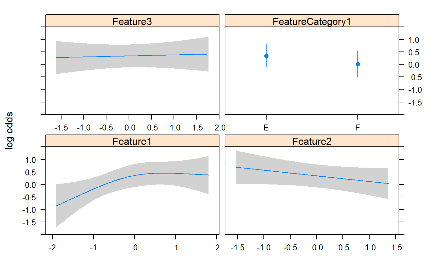
outVar="FeatureYN1"
varForTable=c("Feature1", "Feature2","Feature3","FeatureCategory1")

nonLinearTest(rawData,outVar,varForTable,modelType ="lrm")

     Outcome      X          Formula                         P (Variable) P ( Nonlinear) P (TOTAL)
[1,] "FeatureYN1" "Feature1" "FeatureYN1 ~ rcs(Feature1, 3)" "0.044"      "0.127"        "0.044"  
[2,] "FeatureYN1" "Feature2" "FeatureYN1 ~ rcs(Feature2, 3)" "0.133"      "0.119"        "0.133"  
[3,] "FeatureYN1" "Feature3" "FeatureYN1 ~ rcs(Feature3, 3)" "0.881"      "0.649"        "0.881"

#None of them has non-linear term. But will add nonlinear in the model as an example
#(formulaForModel<-as.formula(paste0(outVar,"~",paste(varForTable, collapse=" + "))))
formulaForModel<-as.formula(FeatureYN1~rcs(Feature1,3)+Feature2+Feature3+FeatureCategory1)
dataForModel<-rawData[,c(outVar,varForTable)]
ddist <- datadist(dataForModel)
options(datadist='ddist')

modelResult <- lrm(formulaForModel, data=rawData)
print(modelResult)

Logistic Regression Model
 
 lrm(formula = formulaForModel, data = rawData)
 
                      Model Likelihood     Discrimination    Rank Discrim.    
                         Ratio Test           Indexes           Indexes       
 Obs           200    LR chi2     10.06    R2       0.065    C       0.600    
  0            100    d.f.            5    g        0.508    Dxy     0.199    
  1            100    Pr(> chi2) 0.0737    gr       1.662    gamma   0.199    
 max |deriv| 1e-12                         gp       0.120    tau-a   0.100    
                                           Brier    0.238                     
 
                    Coef    S.E.   Wald Z Pr(>|Z|)
 Intercept           0.5604 0.3297  1.70  0.0892  
 Feature1            0.7432 0.3274  2.27  0.0232  
 Feature1'          -0.5401 0.3520 -1.53  0.1250  
 Feature2           -0.2257 0.1574 -1.43  0.1514  
 Feature3            0.0406 0.1512  0.27  0.7885  
 FeatureCategory1=F -0.3259 0.2952 -1.10  0.2696

#showOddsRatio2(modelResult)
plot(Predict(modelResult))

#extract p value from results
#http://r.789695.n4.nabble.com/Extracting-P-values-from-the-lrm-function-in-the-rms-library-td2260999.html
pnorm(abs(modelResult$coef/sqrt(diag(modelResult$var))),lower.tail=F)*2

         Intercept           Feature1          Feature1'           Feature2           Feature3 FeatureCategory1=F 
        0.08917042         0.02318681         0.12499723         0.15142348         0.78853165         0.26959283

#more plot
plot(Predict(modelResult,fun=plogis))

plot(Predict(modelResult,Feature1,fun=plogis))

plot(Predict(modelResult,Feature1=sort(dataForModel$Feature1),fun=plogis))

temp=Predict(modelResult,Feature1=sort(dataForModel$Feature1),fun=plogis)
str(temp)

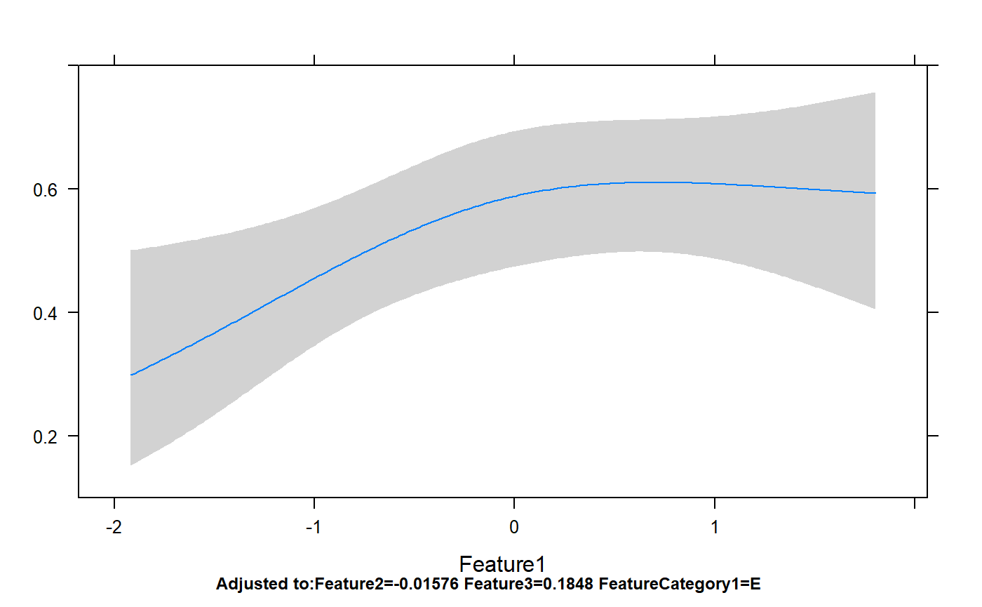
Classes 'Predict' and 'data.frame': 200 obs. of  7 variables:
 $ Feature1        : num  -2.56 -2.36 -2.35 -2.33 -2.28 ...
 $ Feature2        : num  -0.0158 -0.0158 -0.0158 -0.0158 -0.0158 ...
 $ Feature3        : num  0.185 0.185 0.185 0.185 0.185 ...
 $ FeatureCategory1: Factor w/ 2 levels "E","F": 1 1 1 1 1 1 1 1 1 1 ...
 $ yhat            : num  0.209 0.235 0.236 0.238 0.245 ...
 $ lower           : num  0.0714 0.092 0.0932 0.0947 0.1004 ...
 $ upper           : num  0.475 0.482 0.483 0.483 0.485 ...
 - attr(*, "out.attrs")=List of 2
  ..$ dim     : Named int  200 1 1 1
  .. ..- attr(*, "names")= chr  "Feature1" "Feature2" "Feature3" "FeatureCategory1"
  ..$ dimnames:List of 4
  .. ..$ Feature1        : chr  "Feature1=-2.562726" "Feature1=-2.356756" "Feature1=-2.345888" "Feature1=-2.332444" ...
  .. ..$ Feature2        : chr "Feature2=-0.01576"
  .. ..$ Feature3        : chr "Feature3=0.1848"
  .. ..$ FeatureCategory1: chr "FeatureCategory1=E"
 - attr(*, "info")=List of 11
  ..$ varying     : chr "Feature1"
  ..$ adjust      : chr "Feature2=-0.01576 Feature3=0.1848 FeatureCategory1=E "
  ..$ Design      :List of 3
  .. ..$ label      : Named chr  "Feature1" "Feature2" "Feature3" "FeatureCategory1"
  .. .. ..- attr(*, "names")= chr  "Feature1" "Feature2" "Feature3" "FeatureCategory1"
  .. ..$ units      : Named chr  "" "" "" ""
  .. .. ..- attr(*, "names")= chr  "Feature1" "Feature2" "Feature3" "FeatureCategory1"
  .. ..$ assume.code: Named int  4 1 1 5
  .. .. ..- attr(*, "names")= chr  "Feature1" "Feature2" "Feature3" "FeatureCategory1"
  ..$ ylabPlotmath: chr ""
  ..$ ylabhtml    : chr ""
  ..$ ylab        : chr ""
  ..$ yunits      : NULL
  ..$ ref.zero    : logi FALSE
  ..$ adj.zero    : logi FALSE
  ..$ time        : NULL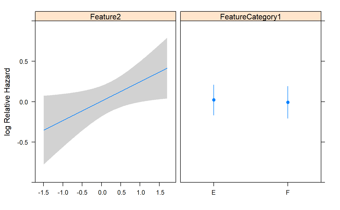
  ..$ conf.int    : num 0.95

p=rms:::ggplot.Predict(temp,ylim=c(0,1))
#same thing
#p=ggplot(temp,aes(x=Feature1,y=yhat),ylim=c(0,1))+geom_line()+geom_ribbon(aes(ymin=lower,ymax=upper),alpha=0.05)

p+geom_point(aes(x=Feature1,y=FeatureYN1),data=dataForModel)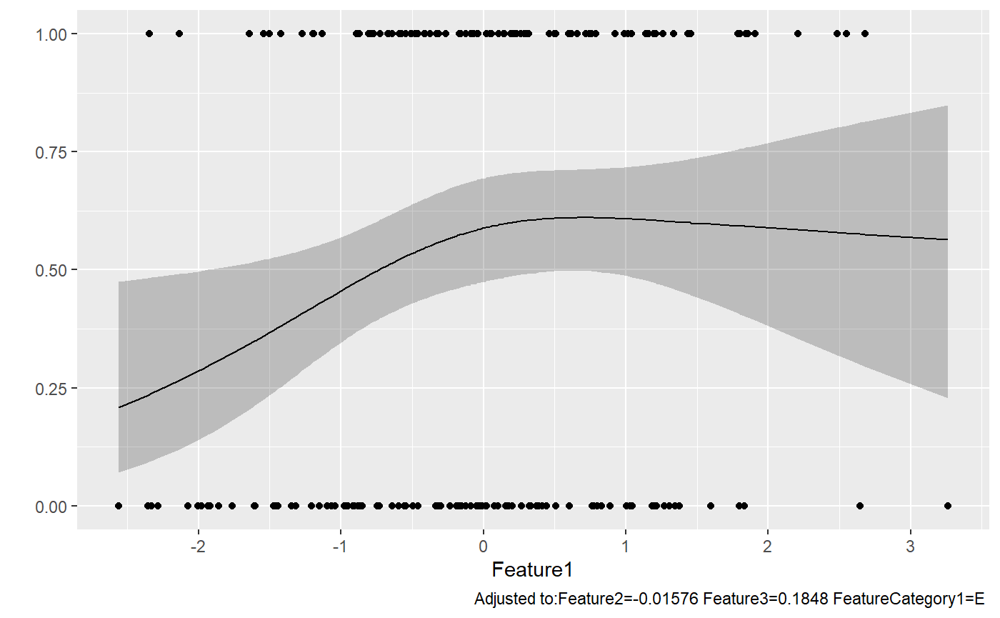

##Logistic regression: ROC curve and best cutoff

Simple one variable model

https://stackoverflow.com/questions/16347507/obtaining-threshold-values-from-a-roc-curve

Or using OptimalCutpoints package which provides many algorithms to find an optimal thresholds. Or coords function in pROC package

source("D:\\source\\r_cqs\\myPkg\\R\\logisticRegressionAndRocFunctions.R")

dataForModel=rawData
temp=makeModelAndTable(dataForModel,labelVar="FeatureYN1",xVar="Feature1")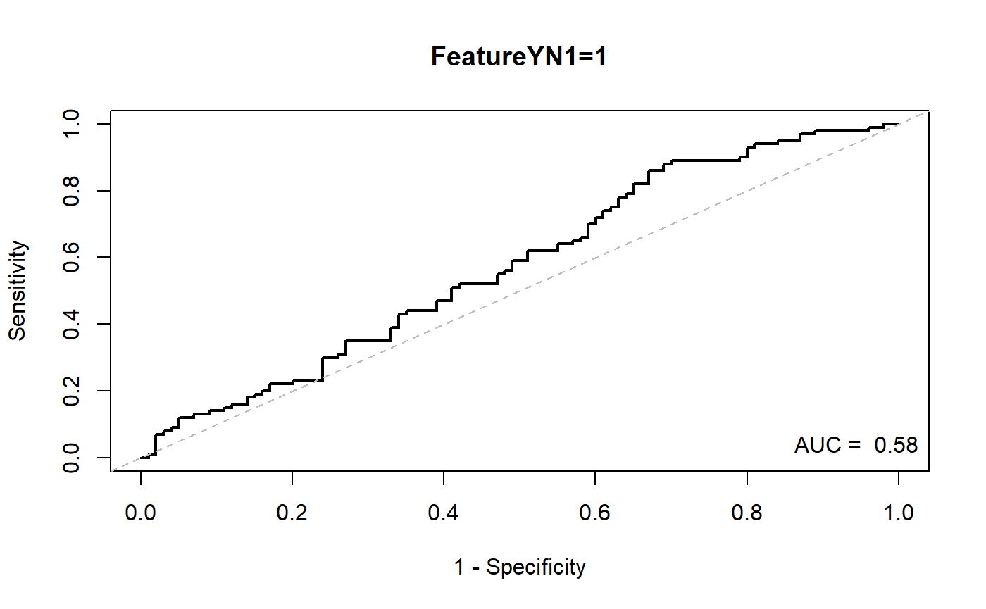

kable(temp)

cut	sens	spec	ppv	npv
-1.44327239102318	0.95	0.15	0.5300000	0.7500000
-0.771357770606852	0.83	0.33	0.5500000	0.6600000
-0.0396971579882457	0.53	0.53	0.5300000	0.5300000
0.744156606775947	0.26	0.76	0.5200000	0.5100000
1.31169924528837	0.13	0.93	0.6500000	0.5200000
Max (Sens+Spec): -0.803291122937887	0.86	0.33	0.5620915	0.7021277
Max Spec when Sens>=0.8: -0.667217415388882	0.80	0.35	0.5517241	0.6363636

Complicated Model

source("D:\\source\\r_cqs\\myPkg\\R\\logisticRegressionAndRocFunctions.R")

otherVar=c("FeatureYN1")
xVarList<-list(
        "Feature1",
        c("Feature2","FeatureCategory1")
)
otherVar=c("Feature3") #like age and gender
plotModelRocAdjusted(dataForModel,
        xVarList=xVarList,outVar=outVar,otherVar=otherVar,
        verbose=TRUE)

## Logistic Regression Model
##  
##  lrm(formula = formulaForModel, data = dataForModel, x = TRUE, 
##      y = TRUE)
##  
##                       Model Likelihood     Discrimination    Rank Discrim.    
##                          Ratio Test           Indexes           Indexes       
##  Obs           200    LR chi2      4.45    R2       0.029    C       0.582    
##   0            100    d.f.            2    g        0.343    Dxy     0.163    
##   1            100    Pr(> chi2) 0.1083    gr       1.409    gamma   0.163    
##  max |deriv| 1e-09                         gp       0.084    tau-a   0.082    
##                                            Brier    0.244                     
##  
##            Coef   S.E.   Wald Z Pr(>|Z|)
##  Intercept 0.0064 0.1439 0.04   0.9647  
##  Feature1  0.2769 0.1342 2.06   0.0391  
##  Feature3  0.0257 0.1491 0.17   0.8632  
##

## Setting levels: control = 0, case = 1

## Setting direction: controls < cases

## Logistic Regression Model
##  
##  lrm(formula = formulaForModel, data = dataForModel, x = TRUE, 
##      y = TRUE)
##  
##                       Model Likelihood     Discrimination    Rank Discrim.    
##                          Ratio Test           Indexes           Indexes       
##  Obs           200    LR chi2      2.67    R2       0.018    C       0.555    
##   0            100    d.f.            3    g        0.264    Dxy     0.109    
##   1            100    Pr(> chi2) 0.4453    gr       1.303    gamma   0.109    
##  max |deriv| 2e-11                         gp       0.065    tau-a   0.055    
##                                            Brier    0.247                     
##  
##                     Coef    S.E.   Wald Z Pr(>|Z|)
##  Intercept           0.1075 0.1923  0.56  0.5763  
##  Feature2           -0.2120 0.1553 -1.37  0.1722  
##  FeatureCategory1=F -0.2653 0.2868 -0.93  0.3549  
##  Feature3            0.0247 0.1487  0.17  0.8681  
##

## Setting levels: control = 0, case = 1
## Setting direction: controls < cases

## Logistic Regression Model
##  
##  lrm(formula = formulaForModel, data = dataForModel, x = TRUE, 
##      y = TRUE)
##  
##                       Model Likelihood     Discrimination    Rank Discrim.    
##                          Ratio Test           Indexes           Indexes       
##  Obs           200    LR chi2      7.65    R2       0.050    C       0.599    
##   0            100    d.f.            4    g        0.453    Dxy     0.198    
##   1            100    Pr(> chi2) 0.1052    gr       1.573    gamma   0.198    
##  max |deriv| 8e-08                         gp       0.109    tau-a   0.099    
##                                            Brier    0.241                     
##  
##                     Coef    S.E.   Wald Z Pr(>|Z|)
##  Intercept           0.1552 0.1961  0.79  0.4288  
##  Feature1            0.3006 0.1376  2.19  0.0289  
##  Feature2           -0.2181 0.1568 -1.39  0.1643  
##  FeatureCategory1=F -0.3481 0.2935 -1.19  0.2357  
##  Feature3            0.0181 0.1501  0.12  0.9039  
##

## Setting levels: control = 0, case = 1
## Setting direction: controls < cases

## Warning in coords.roc(resultRoc[[length(resultRoc)]], "best"): An upcoming version of pROC will set the 'transpose' argument to FALSE by default. Set transpose = TRUE explicitly to keep the current behavior, or transpose = FALSE to adopt the new one and silence this warning. Type help(coords_transpose) for additional information.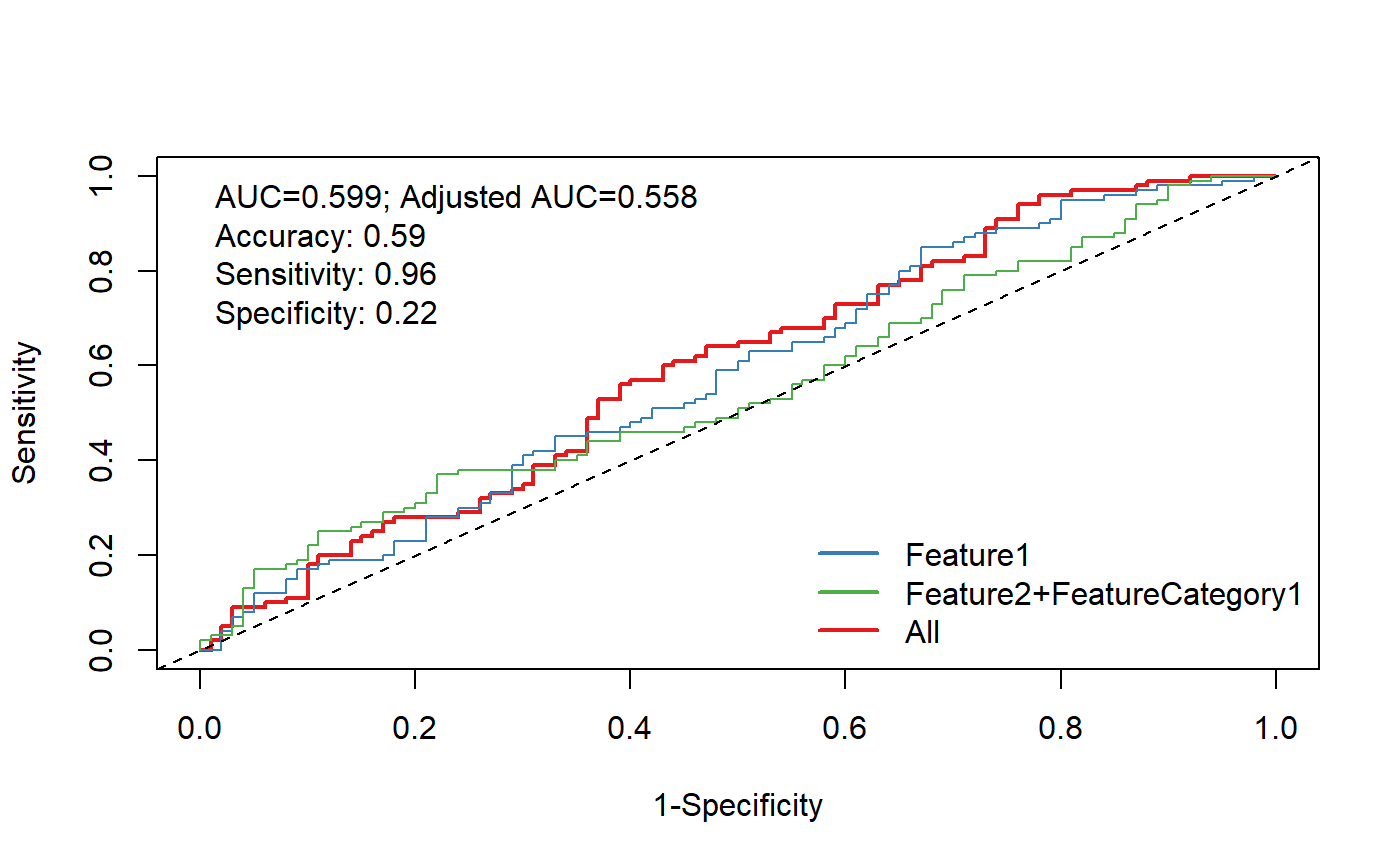

## Confusion Matrix and Statistics
## 
##           Reference
## Prediction  0  1
##          0 22  4
##          1 78 96
##                                           
##                Accuracy : 0.59            
##                  95% CI : (0.5184, 0.6589)
##     No Information Rate : 0.5             
##     P-Value [Acc > NIR] : 0.006565        
##                                           
##                   Kappa : 0.18            
##                                           
##  Mcnemar's Test P-Value : 7.536e-16       
##                                           
##             Sensitivity : 0.9600          
##             Specificity : 0.2200          
##          Pos Pred Value : 0.5517          
##          Neg Pred Value : 0.8462          
##              Prevalence : 0.5000          
##          Detection Rate : 0.4800          
##    Detection Prevalence : 0.8700          
##       Balanced Accuracy : 0.5900          
##                                           
##        'Positive' Class : 1               
##

Linear regression

outVar="Feature1"
varForTable=c("FeatureYN1", "Feature2","Feature3","FeatureCategory1")

nonLinearTest(rawData,outVar,varForTable,modelType ="ols")

     Outcome    X          Formula                       P (Variable) P ( Nonlinear) P (TOTAL)
[1,] "Feature1" "Feature2" "Feature1 ~ rcs(Feature2, 3)" "0.961"      "0.868"        "0.961"  
[2,] "Feature1" "Feature3" "Feature1 ~ rcs(Feature3, 3)" "0.106"      "0.035"        "0.106"

modelTable(rawData,outVars="Feature1",interestedVars=list(c("FeatureYN1"),c("Feature2","FeatureCategory1")),adjVars="Feature3",modelType ="ols")

                                                  Formula          InterestedVar      P Effect (One Unit) Effect (Lower 95%) Effect (Upper 95%) Value (25% Quantile) Value (75% Quantile) Value Diff (75%-25%) Effect (Diff: 75%-25%) Effect (Diff, Lower 95%) Effect (Diff, Upper 95%)
1                  ols (Feature1 ~ FeatureYN1 + Feature3)       FeatureYN1 - 1:0  0.076             0.239             -0.027              0.505                                                                                                                                        
2 ols (Feature1 ~ Feature2 + FeatureCategory1 + Feature3)               Feature2 0.6897            -0.028             -0.169              0.112               -0.555                0.685                 1.24                 -0.035                   -0.209                    0.139
3 ols (Feature1 ~ Feature2 + FeatureCategory1 + Feature3) FeatureCategory1 - F:E 0.0696            -0.244             -0.509              0.021

modelTable(rawData,outVars="Feature1",interestedVars=c("FeatureYN1","Feature2","FeatureCategory1"),adjVars="Feature3",modelType ="ols")

                                       Formula          InterestedVar      P Effect (One Unit) Effect (Lower 95%) Effect (Upper 95%) Value (25% Quantile) Value (75% Quantile) Value Diff (75%-25%) Effect (Diff: 75%-25%) Effect (Diff, Lower 95%) Effect (Diff, Upper 95%)
1       ols (Feature1 ~ FeatureYN1 + Feature3)       FeatureYN1 - 1:0  0.076             0.239             -0.027              0.505                                                                                                                                        
2         ols (Feature1 ~ Feature2 + Feature3)               Feature2 0.8021            -0.018             -0.159              0.123               -0.555                0.685                 1.24                 -0.022                   -0.197                    0.152
3 ols (Feature1 ~ FeatureCategory1 + Feature3) FeatureCategory1 - F:E 0.0732            -0.240             -0.503              0.024

Survival Model

KM Curves

source("D:\\source\\r_cqs\\myPkg\\R\\survivalCurveTable.R")

set.seed(123)
rawData$FeatureAbs1<-abs(rnorm(nrow(rawData))*100)

fit1 <- survfit(Surv(FeatureAbs1, FeatureYN1) ~ FeatureCategory1,data=rawData)
kmplot(fit1,col.surv=1:2,lwd.surv=3,grid=FALSE,las=1,pValue=TRUE,cex.axis=1.2,loc.legend="topright")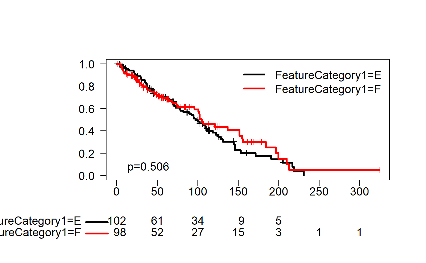

print(fit1)

## Call: survfit(formula = Surv(FeatureAbs1, FeatureYN1) ~ FeatureCategory1, 
##     data = rawData)
## 
##                      n events median 0.95LCL 0.95UCL
## FeatureCategory1=E 102     64   97.7    78.0     122
## FeatureCategory1=F  98     49  104.9    96.2     155

Model

ddist <- datadist(rawData)
options(datadist='ddist')

varForSurvivalModel1=c("FeatureCategory1","Feature2")
(fmla<-as.formula(paste0("Surv(FeatureAbs1, FeatureYN1)~",paste0(varForSurvivalModel1,collapse="+"))))

## Surv(FeatureAbs1, FeatureYN1) ~ FeatureCategory1 + Feature2

fmi=cph(fmla,data=rawData,x=TRUE, y=TRUE)

print(fmi)

## Cox Proportional Hazards Model
##  
##  cph(formula = fmla, data = rawData, x = TRUE, y = TRUE)
##  
##                       Model Tests       Discrimination    
##                                            Indexes        
##  Obs        200    LR chi2      5.05    R2       0.025    
##  Events     113    d.f.            2    Dxy      0.063    
##  Center -0.0066    Pr(> chi2) 0.0799    g        0.259    
##                    Score chi2   4.89    gr       1.296    
##                    Pr(> chi2) 0.0867                      
##  
##                     Coef    S.E.   Wald Z Pr(>|Z|)
##  FeatureCategory1=F -0.0285 0.1964 -0.14  0.8847  
##  Feature2            0.2400 0.1135  2.11  0.0345  
##

#showOddsRatio2(fmi)
plot(Predict(fmi))

validate(fmi) #

##       index.orig training   test optimism index.corrected  n
## Dxy       0.0630   0.1050 0.0614   0.0437          0.0193 40
## R2        0.0252   0.0382 0.0213   0.0169          0.0082 40
## Slope     1.0000   1.0000 0.7995   0.2005          0.7995 40
## D         0.0042   0.0071 0.0034   0.0037          0.0005 40
## U        -0.0021  -0.0021 0.0013  -0.0034          0.0013 40
## Q         0.0063   0.0092 0.0021   0.0071         -0.0008 40
## g         0.2593   0.3122 0.2369   0.0753          0.1840 40

Concordance and C-index

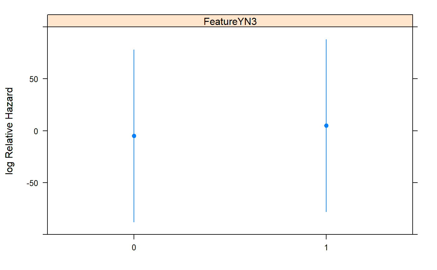
https://stats.stackexchange.com/questions/169834/cox-regression-covariate-specific-concordance-independent-of-distribution-of-cov

testData=data.frame(FeatureYN1=c(0,1),FeatureAbs1=1:10,FeatureYN2=as.factor(rep(c(0,1),each=5)),FeatureAbs2=c(1,2,3,4,5),FeatureYN3=as.factor(c(0,1)),FeatureYN4=as.factor(c(0,0,0,1,0,1,0,1,0,1)))

ddist <- datadist(testData)
options(datadist='ddist')

varForSurvivalModel1=c("FeatureYN3")
(fmla<-as.formula(paste0("Surv(FeatureAbs1, FeatureYN1)~",paste0(varForSurvivalModel1,collapse="+"))))

## Surv(FeatureAbs1, FeatureYN1) ~ FeatureYN3

fmi=cph(fmla,data=testData)

print(fmi)

## Cox Proportional Hazards Model
##  
##  cph(formula = fmla, data = testData)
##  
##                      Model Tests       Discrimination    
##                                           Indexes        
##  Obs        10    LR chi2      4.13    R2       0.453    
##  Events      5    d.f.            1    Dxy      0.500    
##  Center 4.9389    Pr(> chi2) 0.0422    g        5.488    
##                   Score chi2   2.70    gr     241.682    
##                   Pr(> chi2) 0.1001                      
##  
##               Coef   S.E.    Wald Z Pr(>|Z|)
##  FeatureYN3=1 9.8777 84.7068 0.12   0.9072  
##

plot(Predict(fmi))

#Dxy are equal to 2 * (C - 0.5), so C-index=(Dxy+1)/2=0.75

rcorr.cens(testData$FeatureAbs2, Surv(testData$FeatureAbs1, testData$FeatureYN1)) #0.75

##        C Index            Dxy           S.D.              n        missing     uncensored Relevant Pairs     Concordant      Uncertain 
##      0.7500000      0.5000000      0.2397916     10.0000000      0.0000000      5.0000000     40.0000000     30.0000000     50.0000000

fit1 <- coxph(fmla,data=testData)

## Warning in fitter(X, Y, istrat, offset, init, control, weights = weights, : Loglik converged before variable 1 ; coefficient may be infinite.

concordance(fit1) #0.75

## Call:
## concordance.coxph(object = fit1)
## 
## n= 10 
## Concordance= 0.75 se= 0.09682
## concordant discordant     tied.x     tied.y    tied.xy 
##         10          0         10          0          0

library(survcomp)

## Loading required package: prodlim

## Warning: package 'prodlim' was built under R version 3.6.1

concordance.index(x=testData$FeatureAbs2, surv.time=testData$FeatureAbs1, surv.event=testData$FeatureYN1,outx=FALSE) #0.25, if using x=-testData$FeatureAbs2, getting 0.75

## $c.index
## [1] 0.25
## 
## $se
## [1] NA
## 
## $lower
## [1] 0.02907911
## 
## $upper
## [1] 0.7876805
## 
## $p.value
## [1] NA
## 
## $n
## [1] 10
## 
## $data
## $data$x
##  [1] 1 2 3 4 5 1 2 3 4 5
## 
## $data$surv.time
##  [1]  1  2  3  4  5  6  7  8  9 10
## 
## $data$surv.event
##  [1] 0 1 0 1 0 1 0 1 0 1
## 
## 
## $comppairs
## [1] 40

concordance.index(x=testData$FeatureYN3, surv.time=testData$FeatureAbs1,surv.event=testData$FeatureYN1,outx=TRUE)

## $c.index
## [1] NA
## 
## $se
## [1] NA
## 
## $lower
## [1] NA
## 
## $upper
## [1] NA
## 
## $p.value
## [1] NA
## 
## $n
## [1] 10
## 
## $data
## $data$x
##  [1] 0 1 0 1 0 1 0 1 0 1
## Levels: 0 1
## 
## $data$surv.time
##  [1]  1  2  3  4  5  6  7  8  9 10
## 
## $data$surv.event
##  [1] 0 1 0 1 0 1 0 1 0 1
## 
## 
## $comppairs
## [1] 20

concordance.index(x=testData$FeatureYN4, surv.time=testData$FeatureAbs1,surv.event=testData$FeatureYN1,outx=TRUE)

## $c.index
## [1] 0.6
## 
## $se
## [1] NA
## 
## $lower
## [1] 0.08406052
## 
## $upper
## [1] 0.9608096
## 
## $p.value
## [1] NA
## 
## $n
## [1] 10
## 
## $data
## $data$x
##  [1] 0 0 0 1 0 1 0 1 0 1
## Levels: 0 1
## 
## $data$surv.time
##  [1]  1  2  3  4  5  6  7  8  9 10
## 
## $data$surv.event
##  [1] 0 1 0 1 0 1 0 1 0 1
## 
## 
## $comppairs
## [1] 20

##Missing values

Table 0: Missing Data Describe

varForTable=colnames(rawDataWithMissing)
s=describe(rawDataWithMissing[,varForTable])
html(s, exclude1=FALSE,  what=c('%'),digits=3, prmsd=TRUE)

## Warning in png(file, width = 1 + k * w, height = h): 'width=13, height=13' are unlikely values in pixels

rawDataWithMissing[, varForTable]

13 Variables 200 Observations

Feature1

        n  missing distinct     Info     Mean      Gmd      .05      .10      .25 
      191        9      191        1  0.04745    1.075  -1.7758  -1.3315  -0.4751 
      .50      .75      .90      .95 
   0.1021   0.7174   1.2184   1.5383

lowest :	-2.639306	-2.527274	-2.304690	-2.024790	-1.972192
highest:	1.827012	1.907589	1.978721	2.159180	2.345727

Feature2

        n  missing distinct     Info     Mean      Gmd      .05      .10      .25 
      190       10      190        1  0.04649    1.048 -1.44808 -1.13547 -0.52462 
      .50      .75      .90      .95 
  0.07378  0.66921  1.27675  1.69768

lowest :	-2.777412	-2.508263	-2.074123	-1.986896	-1.979580
highest:	1.796271	1.831323	1.849473	2.163419	2.348937

Feature3

         n   missing  distinct      Info      Mean       Gmd       .05       .10 
       185        15       185         1   0.03192     1.156 -1.764851 -1.191339 
       .25       .50       .75       .90       .95 
 -0.597037  0.002022  0.731282  1.457951  1.679656

lowest :	-2.725607	-2.264711	-2.207013	-2.188020	-2.173589
highest:	2.052789	2.102634	2.126548	2.136332	2.310895

Feature4

        n  missing distinct     Info     Mean      Gmd      .05      .10      .25 
      185       15      185        1   0.1263    1.148  -1.4523  -1.1570  -0.5940 
      .50      .75      .90      .95 
   0.1226   0.8695   1.3664   1.8094

lowest :	-2.692560	-2.244344	-1.924571	-1.883894	-1.804621
highest:	2.248268	2.309956	2.320966	2.602364	2.641158

Feature5

        n  missing distinct     Info     Mean      Gmd      .05      .10      .25 
      185       15      185        1 -0.07152    1.154  -1.6226  -1.3590  -0.8384 
      .50      .75      .90      .95 
  -0.1233   0.6871   1.2558   1.7241

lowest :	-2.640512	-2.345108	-2.198916	-1.952043	-1.909586
highest:	1.994208	2.115217	2.148598	2.335518	2.350423

Feature6

        n  missing distinct     Info     Mean      Gmd      .05      .10      .25 
      182       18      182        1  0.05637    1.131 -1.67913 -1.18108 -0.68707 
      .50      .75      .90      .95 
  0.06727  0.74970  1.30356  1.69913

lowest :	-2.360067	-2.320204	-2.044873	-1.888736	-1.881225
highest:	1.913851	1.933405	2.063325	2.241895	2.787574

Feature7

        n  missing distinct     Info     Mean      Gmd      .05      .10      .25 
      182       18      182        1   0.1384      1.1  -1.5849  -1.1785  -0.5250 
      .50      .75      .90      .95 
   0.2155   0.8354   1.2754   1.4682

lowest :	-2.421316	-2.415046	-2.146252	-2.117070	-1.741206
highest:	1.986423	2.105750	2.207151	2.557260	2.619695

Feature8

         n   missing  distinct      Info      Mean       Gmd       .05       .10 
       184        16       184         1 -0.006987     1.038 -1.575089 -1.134838 
       .25       .50       .75       .90       .95 
 -0.611357 -0.005552  0.628806  1.146343  1.375269

lowest :	-2.749489	-2.571196	-2.326160	-2.192145	-2.103843
highest:	1.785670	1.897934	2.017092	2.132327	3.075039

Feature9

        n  missing distinct     Info     Mean      Gmd      .05      .10      .25 
      180       20      180        1  0.07332    1.223 -1.85282 -1.22584 -0.67268 
      .50      .75      .90      .95 
  0.07349  0.71873  1.28070  2.08699

lowest :	-3.161448	-2.641805	-2.512105	-2.327999	-2.233521
highest:	2.520853	2.527255	2.643755	2.895626	2.896421

Feature10

        n  missing distinct     Info     Mean      Gmd      .05      .10      .25 
      184       16      184        1 -0.07797    1.133 -1.85996 -1.48696 -0.70670 
      .50      .75      .90      .95 
 -0.01601  0.59932  1.18404  1.62936

lowest :	-2.477123	-2.403935	-2.272974	-2.261448	-2.046365
highest:	1.845156	1.890087	1.897335	1.919223	2.546919

FeatureYN1

n	missing	distinct	Info	Sum	Mean	Gmd
185	15	2	0.74	103	0.5568	0.4962

FeatureCategory1

n	missing	distinct
188	12	2

 Value          E     F
 Frequency     98    90
 Proportion 0.521 0.479

FeatureCategory2

n	missing	distinct
185	15	4

 Value          A     B     C     D
 Frequency     48    54    53    30
 Proportion 0.259 0.292 0.286 0.162

Missing Value Imputation

dataImputated <- aregImpute(~Feature1+Feature2+Feature3+
                Feature4+Feature5+Feature6+Feature7+Feature8+Feature9+Feature10+
                FeatureYN1+FeatureCategory1+FeatureCategory2,
        n.impute=10, data=rawDataWithMissing, nk=0,x=TRUE)

## Iteration 1 
Iteration 2 
Iteration 3 
Iteration 4 
Iteration 5 
Iteration 6 
Iteration 7 
Iteration 8 
Iteration 9 
Iteration 10 
Iteration 11 
Iteration 12 
Iteration 13

print(dataImputated)

## 
## Multiple Imputation using Bootstrap and PMM
## 
## aregImpute(formula = ~Feature1 + Feature2 + Feature3 + Feature4 + 
##     Feature5 + Feature6 + Feature7 + Feature8 + Feature9 + Feature10 + 
##     FeatureYN1 + FeatureCategory1 + FeatureCategory2, data = rawDataWithMissing, 
##     n.impute = 10, nk = 0, x = TRUE)
## 
## n: 200   p: 13   Imputations: 10     nk: 0 
## 
## Number of NAs:
##         Feature1         Feature2         Feature3         Feature4         Feature5         Feature6         Feature7         Feature8         Feature9        Feature10       FeatureYN1 FeatureCategory1 FeatureCategory2 
##                9               10               15               15               15               18               18               16               20               16               15               12               15 
## 
##                  type d.f.
## Feature1            l    1
## Feature2            l    1
## Feature3            l    1
## Feature4            l    1
## Feature5            l    1
## Feature6            l    1
## Feature7            l    1
## Feature8            l    1
## Feature9            l    1
## Feature10           l    1
## FeatureYN1          l    1
## FeatureCategory1    c    1
## FeatureCategory2    c    3
## 
## Transformation of Target Variables Forced to be Linear
## 
## R-squares for Predicting Non-Missing Values for Each Variable
## Using Last Imputations of Predictors
##         Feature1         Feature2         Feature3         Feature4         Feature5         Feature6         Feature7         Feature8         Feature9        Feature10       FeatureYN1 FeatureCategory1 FeatureCategory2 
##            0.146            0.087            0.131            0.165            0.138            0.115            0.091            0.187            0.183            0.108            0.119            0.112            0.191

#Values after imputation
names(dataImputated$imputed)

##  [1] "Feature1"         "Feature2"         "Feature3"         "Feature4"         "Feature5"         "Feature6"         "Feature7"         "Feature8"         "Feature9"         "Feature10"        "FeatureYN1"       "FeatureCategory1" "FeatureCategory2"

tail(dataImputated$imputed$Feature1)

##                 [,1]        [,2]         [,3]       [,4]       [,5]       [,6]       [,7]        [,8]        [,9]       [,10]
## Sample163 -1.9252795  0.07161431  1.530290893 -2.3046903 -1.8625206 -0.5475122 -1.3314980 -0.12369319 -0.06305878 -0.44084254
## Sample170  0.5343689 -1.63741841  0.175195465 -0.2965603 -0.4217670 -0.1800521 -0.9919236  0.02631987  0.07871215 -1.94313607
## Sample176  0.8092622 -0.47498252 -0.007745175  1.5373611  0.6679670 -0.1323495  0.3669057  0.84124489 -0.09101177  0.42978724
## Sample179 -0.6881552 -0.78933020  0.260467527  0.6679670  1.7061845  0.1296105  0.6679670  1.53029089  1.70618451  1.70618451
## Sample194 -0.4107861 -0.03540051 -0.273904423 -0.4107861  0.7228018  0.4028824 -1.5930815  0.23486904  0.40288242  0.02631987
## Sample199  0.8980107  0.20889323  0.802823332 -0.4107861  1.0767401  0.8028233 -0.5213969 -0.44388628  0.71201736  0.76203875

Model after Missing Value Imputation

fmi <- fit.mult.impute(FeatureYN1~Feature1+Feature2+Feature3+FeatureCategory2,
        lrm, dataImputated,  
#       subset=which(rawDataWithMissing$FeatureCategory1=="E"),
        data=rawDataWithMissing)

## 
## Variance Inflation Factors Due to Imputation:
## 
##          Intercept           Feature1           Feature2           Feature3 FeatureCategory2=B FeatureCategory2=C FeatureCategory2=D 
##               1.07               1.22               1.12               1.39               1.11               1.11               1.23 
## 
## Rate of Missing Information:
## 
##          Intercept           Feature1           Feature2           Feature3 FeatureCategory2=B FeatureCategory2=C FeatureCategory2=D 
##               0.07               0.18               0.11               0.28               0.10               0.10               0.19 
## 
## d.f. for t-distribution for Tests of Single Coefficients:
## 
##          Intercept           Feature1           Feature2           Feature3 FeatureCategory2=B FeatureCategory2=C FeatureCategory2=D 
##            2092.07             280.19             735.03             114.01             897.40             868.80             259.75 
## 
## The following fit components were averaged over the 10 model fits:
## 
##   stats linear.predictors

print(fmi)

## Logistic Regression Model
##  
##  fit.mult.impute(formula = FeatureYN1 ~ Feature1 + Feature2 + 
##      Feature3 + FeatureCategory2, fitter = lrm, xtrans = dataImputated, 
##      data = rawDataWithMissing)
##  
##                       Model Likelihood     Discrimination    Rank Discrim.    
##                          Ratio Test           Indexes           Indexes       
##  Obs           200    LR chi2      8.47    R2       0.055    C       0.621    
##   0             90    d.f.            6    g        0.481    Dxy     0.243    
##   1            110    Pr(> chi2) 0.2334    gr       1.620    gamma   0.243    
##  max |deriv| 3e-08                         gp       0.115    tau-a   0.120    
##                                            Brier    0.237                     
##  
##                     Coef    S.E.   Wald Z Pr(>|Z|)
##  Intercept           0.3104 0.2981  1.04  0.2978  
##  Feature1            0.2833 0.1707  1.66  0.0969  
##  Feature2            0.2428 0.1701  1.43  0.1535  
##  Feature3           -0.0304 0.1684 -0.18  0.8567  
##  FeatureCategory2=B  0.1170 0.4185  0.28  0.7799  
##  FeatureCategory2=C -0.3719 0.4167 -0.89  0.3722  
##  FeatureCategory2=D -0.2597 0.5091 -0.51  0.6100  
##

##Some notes for Hmisc/rms package

library(scales)
ggplot(Predict(gls1))
print("Exp")

p<-ggplot(Predict(gls1),flipxdiscrete=FALSE,sepdiscrete="list",ylim(3,6))
p[[1]]
p[[1]]+scale_y_continuous(trans="exp",limits = c(3,6))

exp_format <- function() {
     function(x) format(exp(x),digits = 2) 
}
p[[1]]+scale_y_continuous(trans="exp",limits = c(3,6),labels = exp_format())
p[[1]]+scale_y_continuous(labels = exp_format())


p[[2]]
p[[2]]+scale_x_continuous(trans="exp")


ggplot(Predict(gls1),flipxdiscrete=FALSE,addlayer=scale_y_continuous(trans="exp",labels=function(x) round(exp(x),2)))
ggplot(Predict(gls1),flipxdiscrete=FALSE)+coord_trans(y = "exp")

Two-Way ANOVA with Repeated Measures

https://biostats.w.uib.no/factorial-repeated-measures-anova-two-way-repeated-measures-anova/ http://psych.wisc.edu/moore/Rpdf/610-R9_Within2way.pdf https://datascienceplus.com/two-way-anova-with-repeated-measures/

rat.weight <- c(166,168,155,159,151,166,170,160,162,153,220,230,223,233,229,262,274,267,283,274,261,275,264,280,282,343,354,351,359,349,297,311,305,315,303,375,399,388,405,395)
rat.strain <- as.factor(rep(c(rep("strainA",5),rep("strainB",5)),4))
rat.ID <- as.factor(rep(c("rat01","rat02","rat03","rat04","rat05","rat06","rat07","rat08","rat09","rat10"),4))
time.point <- as.factor(c(rep("week08",10), rep("week12",10), rep("week16",10), rep("week20",10)))
my.dataframe <- data.frame(rat.ID,rat.strain,time.point,rat.weight)
head(my.dataframe)

##   rat.ID rat.strain time.point rat.weight
## 1  rat01    strainA     week08        166
## 2  rat02    strainA     week08        168
## 3  rat03    strainA     week08        155
## 4  rat04    strainA     week08        159
## 5  rat05    strainA     week08        151
## 6  rat06    strainB     week08        166

with(my.dataframe, interaction.plot(time.point, rat.ID, rat.weight, pch=c(rep(1,5), rep(2,5)), type="b", col=c("black", "red", "blue", "green", "purple", "orange", "grey", "darkblue", "pink", "darkred"), lty= c(1,2,3,4,5,6,7,8,9,10)))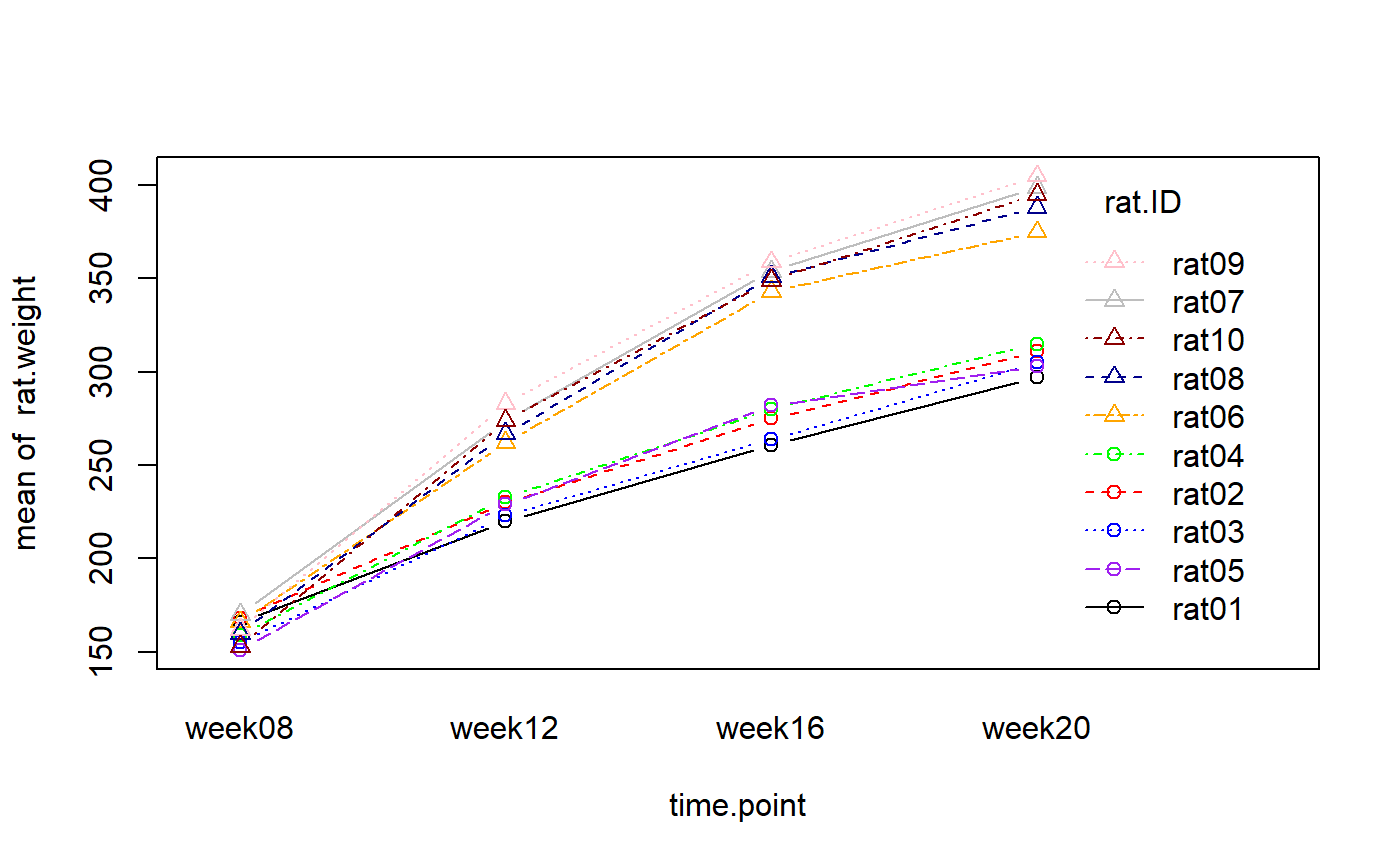

#we need to check for normality of distribution with the Shapiro-Wilk test:
shapiro.test(rat.weight[time.point=="week08" & rat.strain=="strainA"])

## 
##  Shapiro-Wilk normality test
## 
## data:  rat.weight[time.point == "week08" & rat.strain == "strainA"]
## W = 0.94153, p-value = 0.6768

Two-Way ANOVA with Repeated Measures in dataset1

results <- aov(rat.weight~time.point*rat.strain + Error(rat.ID/time.point), data=my.dataframe)
summary(results)

## 
## Error: rat.ID
##            Df Sum Sq Mean Sq F value   Pr(>F)    
## rat.strain  1  28196   28196   217.5 4.39e-07 ***
## Residuals   8   1037     130                     
## ---
## Signif. codes:  0 '***' 0.001 '**' 0.01 '*' 0.05 '.' 0.1 ' ' 1
## 
## Error: rat.ID:time.point
##                       Df Sum Sq Mean Sq F value   Pr(>F)    
## time.point             3 203193   67731  1750.5  < 2e-16 ***
## time.point:rat.strain  3  10980    3660    94.6 1.96e-13 ***
## Residuals             24    929      39                     
## ---
## Signif. codes:  0 '***' 0.001 '**' 0.01 '*' 0.05 '.' 0.1 ' ' 1

A linear mixed-effects model with nested random effects. As a validation.

The F value is the same as Two-Way ANOVA above

library(nlme)

results.lme <- lme(rat.weight~time.point*rat.strain, random=~1|rat.ID, data=my.dataframe)
anova(results.lme)

##                       numDF denDF   F-value p-value
## (Intercept)               1    24 22147.089  <.0001
## time.point                3    24  1750.535  <.0001
## rat.strain                1     8   217.521  <.0001
## time.point:rat.strain     3    24    94.598  <.0001

Two-Way ANOVA with Repeated Measures in dataset2

set.seed(5250)

myData <- data.frame(PID = rep(seq(from = 1,
                               to = 50, by = 1), 20),
                     stress = sample(x = 1:100,
                                     size = 1000,
                                     replace = TRUE),
                     image = sample(c("Happy", "Angry"),
                                    size = 1000,
                                    replace = TRUE),
                     music = sample(c("Disney", "Horror"),
                                    size = 1000,
                                    replace = TRUE)
)

myData <- within(myData, {
  PID   <- factor(PID)
  image <- factor(image)
  music <- factor(music)
})

myData <- myData[order(myData$PID), ]
head(myData)

##     PID stress image  music
## 1     1     90 Angry Disney
## 51    1     42 Angry Disney
## 101   1     84 Angry Horror
## 151   1     10 Angry Horror
## 201   1      5 Angry Disney
## 251   1     34 Happy Disney

#Extracting Condition Means
myData.mean <- aggregate(myData$stress,
                      by = list(myData$PID, myData$music,
                              myData$image),
                      FUN = 'mean')

colnames(myData.mean) <- c("PID","music","image","stress")

myData.mean <- myData.mean[order(myData.mean$PID), ]
head(myData.mean)

##     PID  music image stress
## 1     1 Disney Angry   44.5
## 51    1 Horror Angry   51.5
## 100   1 Disney Happy   49.8
## 149   1 Horror Happy   51.6
## 2     2 Disney Angry   38.5
## 52    2 Horror Angry   28.2

#Building the ANOVA
stress.aov1 <- with(myData.mean,
                   aov(stress ~ music * image +
                       Error(PID / (music * image)))
)

## Warning in aov(stress ~ music * image + Error(PID/(music * image))): Error() model is singular

summary(stress.aov1)

## 
## Error: PID
##             Df Sum Sq Mean Sq F value Pr(>F)  
## music        1    739   739.5   5.171 0.0276 *
## music:image  1    707   706.7   4.942 0.0311 *
## Residuals   47   6721   143.0                 
## ---
## Signif. codes:  0 '***' 0.001 '**' 0.01 '*' 0.05 '.' 0.1 ' ' 1
## 
## Error: PID:music
##             Df Sum Sq Mean Sq F value Pr(>F)
## music        1     13    12.6   0.060  0.808
## image        1    164   163.8   0.774  0.383
## music:image  1    295   295.1   1.395  0.244
## Residuals   47   9943   211.6               
## 
## Error: PID:image
##             Df Sum Sq Mean Sq F value Pr(>F)
## image        1     20   20.18   0.109  0.743
## music:image  1    282  282.10   1.524  0.223
## Residuals   48   8884  185.08               
## 
## Error: PID:music:image
##             Df Sum Sq Mean Sq F value Pr(>F)
## music:image  1     43   43.13   0.214  0.646
## Residuals   47   9457  201.21

stress.aov2 <- with(myData,
                   aov(stress ~ music * image +
                       Error(PID / (music * image)))
)

## Warning in aov(stress ~ music * image + Error(PID/(music * image))): Error() model is singular

summary(stress.aov2)

## 
## Error: PID
##             Df Sum Sq Mean Sq F value  Pr(>F)   
## music        1     33      33   0.056 0.81398   
## image        1    777     777   1.312 0.25795   
## music:image  1   5452    5452   9.211 0.00395 **
## Residuals   46  27229     592                   
## ---
## Signif. codes:  0 '***' 0.001 '**' 0.01 '*' 0.05 '.' 0.1 ' ' 1
## 
## Error: PID:music
##             Df Sum Sq Mean Sq F value Pr(>F)  
## music        1    193     193   0.252 0.6177  
## image        1     37      37   0.049 0.8262  
## music:image  1   3622    3622   4.731 0.0347 *
## Residuals   47  35982     766                 
## ---
## Signif. codes:  0 '***' 0.001 '**' 0.01 '*' 0.05 '.' 0.1 ' ' 1
## 
## Error: PID:image
##             Df Sum Sq Mean Sq F value Pr(>F)
## image        1    297   297.0   0.396  0.532
## music:image  1      5     5.4   0.007  0.933
## Residuals   48  36038   750.8               
## 
## Error: PID:music:image
##             Df Sum Sq Mean Sq F value Pr(>F)
## music:image  1    179   179.1   0.208  0.651
## Residuals   47  40557   862.9               
## 
## Error: Within
##            Df Sum Sq Mean Sq F value Pr(>F)
## Residuals 802 693006   864.1

stress.aov3 <- with(myData,
                   aov(stress ~ music * image +
                       Error(PID/music))
)
summary(stress.aov3)

## 
## Error: PID
##             Df Sum Sq Mean Sq F value  Pr(>F)   
## music        1     33      33   0.056 0.81398   
## image        1    777     777   1.312 0.25795   
## music:image  1   5452    5452   9.211 0.00395 **
## Residuals   46  27229     592                   
## ---
## Signif. codes:  0 '***' 0.001 '**' 0.01 '*' 0.05 '.' 0.1 ' ' 1
## 
## Error: PID:music
##             Df Sum Sq Mean Sq F value Pr(>F)  
## music        1    193     193   0.252 0.6177  
## image        1     37      37   0.049 0.8262  
## music:image  1   3622    3622   4.731 0.0347 *
## Residuals   47  35982     766                 
## ---
## Signif. codes:  0 '***' 0.001 '**' 0.01 '*' 0.05 '.' 0.1 ' ' 1
## 
## Error: Within
##              Df Sum Sq Mean Sq F value Pr(>F)
## image         1    297   297.0   0.347  0.556
## music:image   1    183   183.1   0.214  0.644
## Residuals   898 769602   857.0

stress.aov4 <- aov(stress~music * image + Error(PID/music), data=myData)
summary(stress.aov4)

## 
## Error: PID
##             Df Sum Sq Mean Sq F value  Pr(>F)   
## music        1     33      33   0.056 0.81398   
## image        1    777     777   1.312 0.25795   
## music:image  1   5452    5452   9.211 0.00395 **
## Residuals   46  27229     592                   
## ---
## Signif. codes:  0 '***' 0.001 '**' 0.01 '*' 0.05 '.' 0.1 ' ' 1
## 
## Error: PID:music
##             Df Sum Sq Mean Sq F value Pr(>F)  
## music        1    193     193   0.252 0.6177  
## image        1     37      37   0.049 0.8262  
## music:image  1   3622    3622   4.731 0.0347 *
## Residuals   47  35982     766                 
## ---
## Signif. codes:  0 '***' 0.001 '**' 0.01 '*' 0.05 '.' 0.1 ' ' 1
## 
## Error: Within
##              Df Sum Sq Mean Sq F value Pr(>F)
## image         1    297   297.0   0.347  0.556
## music:image   1    183   183.1   0.214  0.644
## Residuals   898 769602   857.0

library(nlme)
stress.lme0 <- lme(stress~music*image, random=~1|PID, data=myData.mean)
anova(stress.lme0)

##             numDF denDF   F-value p-value
## (Intercept)     1   145 2581.7961  <.0001
## music           1   145    0.1370  0.7118
## image           1   145    0.1314  0.7175
## music:image     1   145    0.4198  0.5181

stress.lme1 <- lme(stress~music*image, random=~1|PID, data=myData)
anova(stress.lme1)

##             numDF denDF   F-value p-value
## (Intercept)     1   947 2924.4077  <.0001
## music           1   947    0.1798  0.6716
## image           1   947    0.7269  0.3941
## music:image     1   947    0.3023  0.5826

stress.lme2 <- lme(stress~music*image, random=~image|PID, data=myData)
anova(stress.lme2)

##             numDF denDF   F-value p-value
## (Intercept)     1   947 2924.4077  <.0001
## music           1   947    0.1798  0.6716
## image           1   947    0.7269  0.3941
## music:image     1   947    0.3023  0.5826

Shilin Zhao

26 June, 2020